bulk-online, the Powder/Bulk Portal

(From the archive of ”bulk solids handling", article published in Vol. 36 (2016) No. 2/3 , ©2016 bulk-online.com)

1. Introduction

Rules and probabilities are the bases of stochastic methods for describing phenomena, they do not have a foundation on a physical principle that “forces” the math to produce the right results (for example the Finite Element Method minimising potential energy to derive the equations used to solve the problem). Stochastic models for gravity flow use just conservation of mass.Despite the weak formulation, stochastic methods can be very powerful tools to solve material flow problems, and some of the merits, limitations and pitfalls of these methods are explored in this paper.

2. Description of the program MFlow

Stochastic methods are modelling tools for estimating outcomes by allowing for random variations in one or more inputs over time. When material is removed from a drawpoint, a void is created that is filled with material from above the void. The exact source of that material is unknown; therefore a random location is assigned.

Fig. 1: Plan view of basic cube grid. (Pictures: © W.H. Gibson)

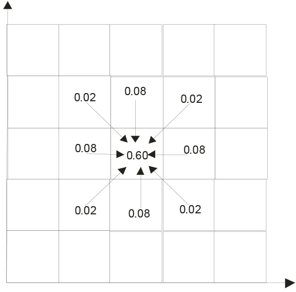
Fig. 1 shows a plan view of a grid describing this concept. When part of the material is removed from a cell below the centre of the grid, the void is filled from any of the nine cells above, as shown on Fig. 1. This process is random, making stochastic models ideal for this type of problem solving. In this particular case, a probability is assigned to each cell indicating the chances that the void will be filled with material from the cell immediately above (60%) or any of the surrounding cells (8% chance cells with adjacent sides and 2% for cells with adjacent corners; percentages given as an example only).The grid shown in Fig. 1 does not match the axisymmetric nature of the problem; a better grid is shown in Fig. 2. This type of grid is better for analysing material flow because the grid can model naturally an axisymmetric problem. The disadvantage of this type of grid is the shape of the cells, which complicates the calculation.

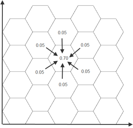Fig. 2: Plan view of hexagonal prisms grid.

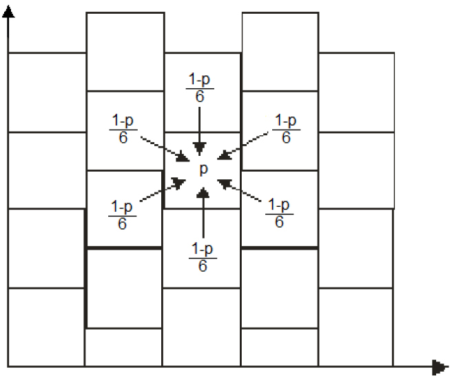Fig. 3: Plan view of cube shifted grid.

Fig. 3 shows a grid that combine the simple geometry of cubes and the circular location of hexagonal prisms. MFlow uses this configuration of cells. p represents the probability that material will be transferred from the cell above. (1-p)/6 is the probability that one of the cells around the central cell can transfer material to the void below.

3. Pascal “Cone” and Correlation between Probabilities andEllipsoid Width

The Pascal triangle can be used to understand how probabilities can be used to assess material flow in 2D. The concept is extended to a 3D (Pascal Cone) to model the gravity flow in three dimensions.

3.1 Model in 2 Dimensions

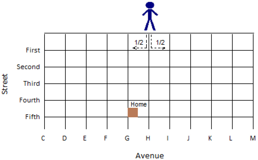
The Pascal triangle can be used to assess the probability that a drunken man can reach home (depicted by the shaded box in Fig. 4), starting in a particular street and walking randomly (Harr 1987). At every corner, there is a 50% chance that the man will turn either left or right. From Fig. 5, it is possible to see the probability of reaching home is 5/16.

Fig. 4: 2D random walk (after Harr 1987).

Fig. 5: Probabilities associated with 2D random walk.

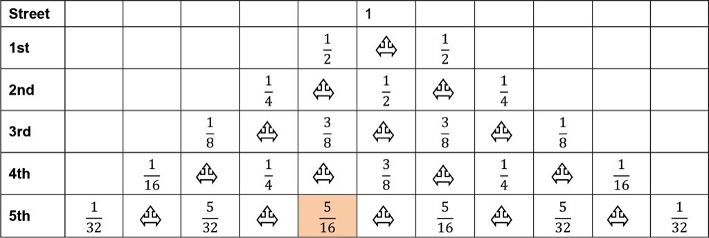
In general, the probability of reaching corner r at street n can be calculated as follows:The probabilistic analysis indicates the chances of the man ending some blocks away from home. The actual distance between the man and his home will depend on the size of the city blocks. The same problem occurs in material flow as is explained the following paragraphs.Fig. 5 presents the probabilities associated with this 2D random walk. If we imagine Fig. 5 upside down, we can see that the value indicated in any cell represents the probability of a cell being affected by extraction of the cell with probability 1 (now at the bottom). This is a very simplistic 2D model where each cell has only two cells above with equal probability to fill the void generated in the cell below, in this case, the chance that the cell highlighted in Fig. 5 is affected by the extraction is 5/16. We can say, after this analysis, that the cell affected is one (1) cell to the left of the cell of extraction but the actual distance of this cell to the extraction point will be a function of the cell size.

Fig. 6: Probabilities within a simple 2D model.

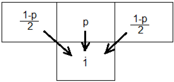
A 2D model can be built with only three (3) cells that can transfer material to cells below. With this simple model, it is possible to study the impact of the parameter p on the ellipsoid of extraction. Fig. 6 presents a vertical section showing probabilities that each cell will transfer material to the cell below. When this concept is applied in a 2D problem, it is possible to assess the chances that a particular cell will be affected by the extraction.

Fig. 7: Probability of material being mobilised for parameter p = 0.7 and p = 0.4.

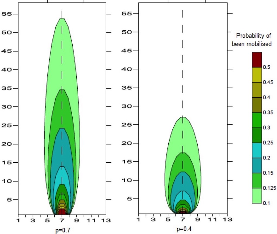
Fig. 7 presents a cross section with a single draw located at x = 7 m. It shows the probability that material located above the drawpoint is mobilised during extraction. The results are presented for two values of p – 0.40 and 0.70. In both cases, the same amount of material is removed from each drawpoint.It is possible to observe that the parameter p controls the width and height of the ellipsoid of extraction. A p value closer to 1 produces a narrower ellipsoid of extraction than a smaller p value. A correlation between p and the actual width of the ellipsoid of extraction is discussed later.The real challenge is in 3D where the calculations of the probabilities are more complicated. If Fig. 3 is used as a reference, then there are seven (7) cells that can fill the void in the cell below and the probabilities for each of the cells are not the same.

3.2 Model in 3 Dimensions

The 3D problem can be viewed not as a Pascal triangle, but more as an inverted “Pascal cone”. It starts with a cell with probability of 1 (certainly we will remove material from there) and the next layer above represent the probability that one cell will fill the void created below. As we move up a layer and more cells are involved in the calculation, the width of interaction between cells is controlled by the value of the probability p indicated in Fig. 3.A similar calculation can be carried out for the 3D case. With this calculation, it is possible to evaluate the diameter of the ellipsoid of extraction for different values of p, as shown in Fig. 8. Note that the width is expressed in number of cells affected by the extraction, and not in actual distance measured in metres.

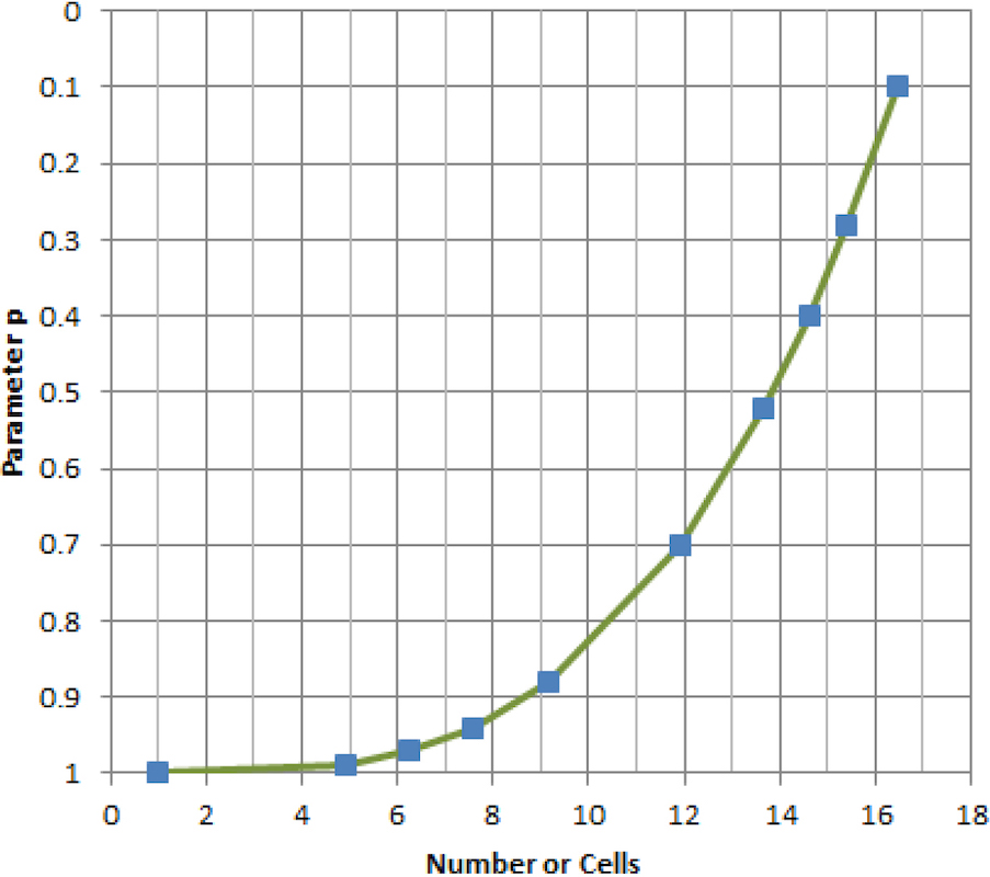Fig. 8: Width of ellipsoid of material mobilised as a function of p.

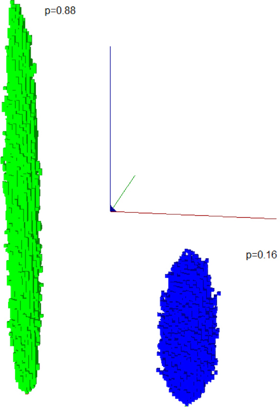Fig. 9: Extraction column width for different p parameters.

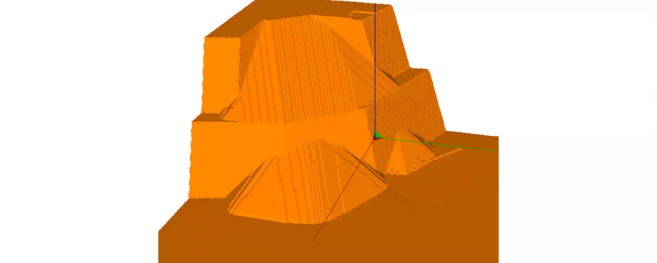
This effect can be visualised on a 3D model of two independent drawpoints in uniform material. Fig. 9 shows the mobilised ellipsoids, clearly illustrating the effect of parameter p on the width of the ellipsoid of extraction. This is an observed behaviour that, depending on physical properties of the broken rock, is controlled by the width for the ellipsoid of extraction.

3.3 Calibration of Parameter p with observed Material Behaviour

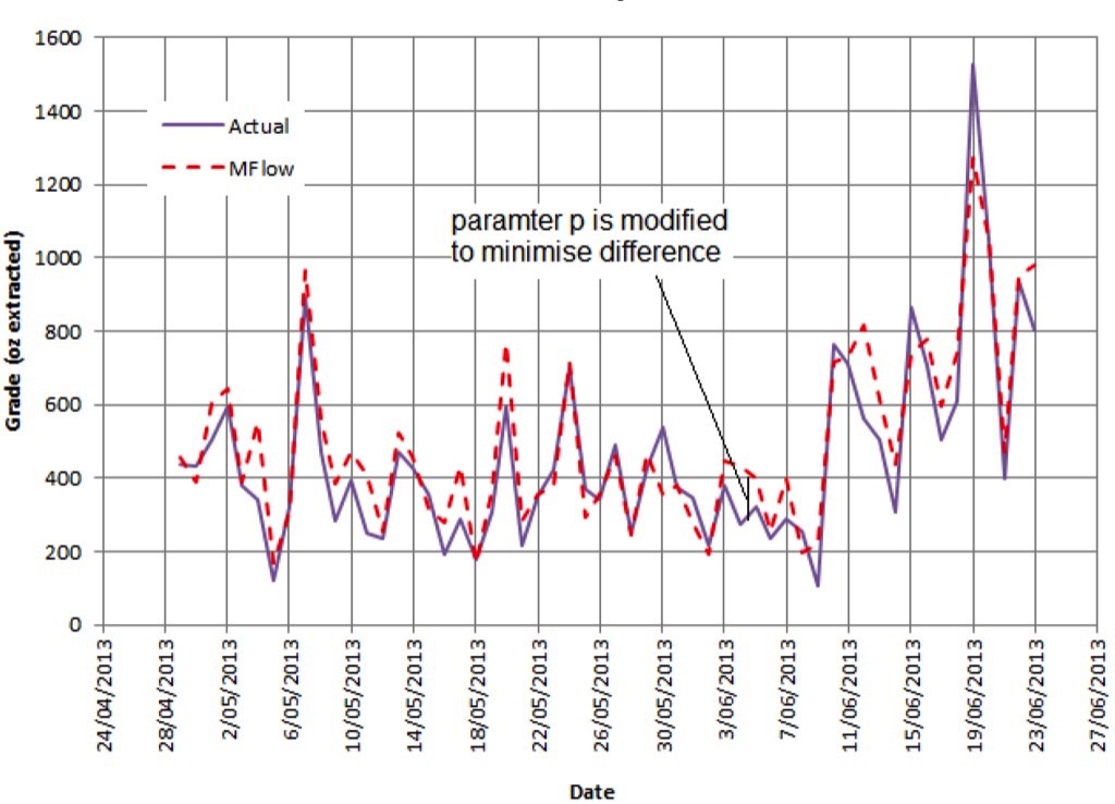
It was shown that in these types of stochastic models, the cell size plays a role in the results; therefore the selection of the cell size has to be made considering other parameters in the model to be able to reproduce the phenomena that have actually been observed.The parameter p controls the width or diameter of the draw column in the model (not the actual length in metres, but the number of cells that will be affected by the draw). If the width of the ellipsoid of extraction is known, it is possible to select a cell size and a probability p to be used in the model.The question that remains is how to relate the rock mass condition or other observed behaviour to parameter p in order to build models that represent the actual material flow.There have been some attempts to relate rock mass condition to ellipsoid width. Laubscher relates the width of the ellipsoid with rock mass classification: the better the rock quality, the wider the ellipsoid (Laubscher 1994). Kvapil recognised the same fact – that an increase in the rock mass quality increases the ellipsoid width (Kvapil 2008).Sharrock (2008) made a review of several aspects of isolated draw and discusses the results of scaled models. Unfortunately, the scaled models did not capture changes in ellipsoid width with material properties or particle size. Susaeta (2004) presented a correlation between friction angle, particle size and ellipsoid width.For mines in operation, it is possible to use information collected from the previous extraction to calibrate p. Fig. 10 shows the ounces extracted in a period of time compared with the values predicted using an MFlow model. The parameter p was modified to minimise the difference between the curves and then calibrated values were used in the future forecasting models.

Fig. 10: Ore extracted used to calibrate parameter p.

There are some guidelines to correlate observed material behaviour with ellipsoid width and this can be used to define parameter p for a given cell size (using Fig. 8). The process of assessing ellipsoid width is based heavily on experience and observations, and less on a strong formulation including the characteristics of the material. Nevertheless, there are some guidelines that can be used to build the stochastic model.

4. Stochastic Modelling Capabilities

Despite the simplicity of the formulation of stochastic models, they can address complex behaviour of materials. Some of these are shown and discussed in the following paragraphs.

4.1 Variable Flow of different Materials (w Factor)

Several factors allow for some materials to travel faster than others in the draw column (Hashim 2009). This type of phenomenon can be included in the model by introducing a weighting factor, w, that modifies the probability of material moving from one cell to another.A value of w = 0 renders the material unaffected by draw and it does not flow. This can be used to define the limits of the draw rings in SLC (Sub Level Caving) if it is assumed that the outside of the blasted ring will not move. A value of w = 1 allows the material to move freely.

Fig. 11: Section of simple model with different materials.

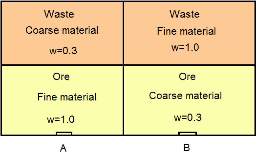
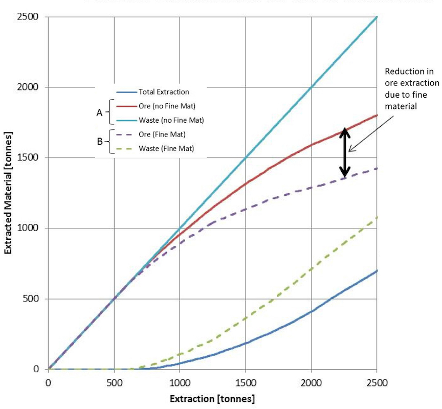
Values between 0 and 1 can therefore be used to control the speed of material flow in the model. To show the effect of the parameter w on the results, the model shown in Fig. 11 was built. Above the extraction point A there is fine ore under coarse waste, above the extraction point B the fine material is on top.The results are shown in Fig. 12. Due to fine waste material, there is a reduction in ore extraction in drawpoint B which is due to a higher dilution of fine material travelling faster than the ore.

Fig. 12: Effect of fine material on extraction.

4.2 Markers

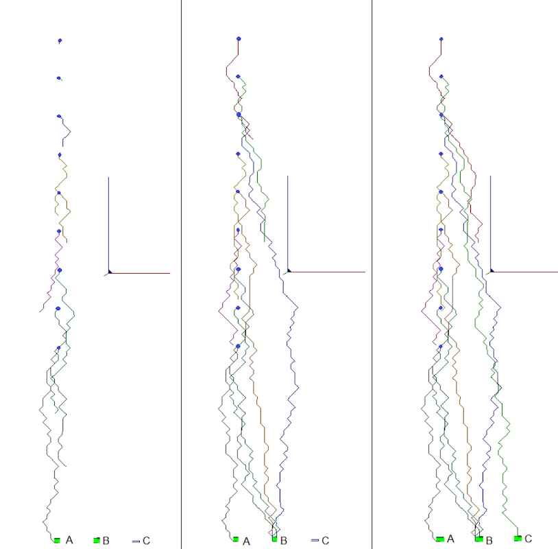
The formulation on stochastic models is easy and that simplicity allows us to incorporate additional calculation into the analysis without adding complexity to the overall analysis. In this case, markers are added in the model to track the movement of the material.Fig. 13 shows the trajectory of markers located above drawpoint A. The sequence of extraction is A then B then C. It is possible to see the change in trajectory of some of the markers and to compare the nature of material that is extracted at the drawpoints.

Fig. 13: Effect of fine material on extraction.

4.3 Finger Path (void diffusion)

Fig. 14: Finger path for a single draw point.

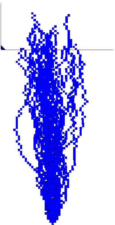
It has been observed that an ellipsoid shaped extraction column is not always generated, and that material can flow following a “finger path” - reaching surface earlier than expected (Brown 2003). This can be simulated by modifying the weighting factor w and giving a higher probability of movement to material already mobilised, as shown in Fig. 14 for a single drawpoint.

4.4 Modelling Surface Flow

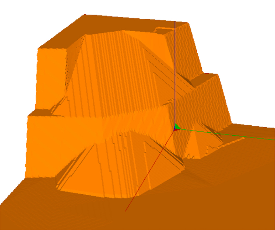
Surface flow or unconfined flow is controlled by the repose angle; the material will flow until the repose angle is reached. This introduces another constraint for the geometry, driven by material properties. Castro(2009) mentioned that in order to model the surface flow the height (h) and the side length of the cells (L) should follow the relationship h/L = tanf where f is the angle of repose. Fig. 15 illustrates a failure on a bench and flow of the loose material.

Fig. 15: Surface flow.

5. Conclusions

Stochastic models have a much easier formulation than other methods such as the Finite Element Method. However, the lack of formulation based on a physical principle makes them more difficult to set up unless information about the rock mass to be modelled is available, thus enabling the modeller to calibrate the model.The results are cell size dependant; therefore cell size has to be selected along with other parameters (probabilities) to ensure the model best represents the material behaviour observed.It is suggested to calibrate a model using the ellipsoid of extraction width estimated from rock mass characterisation or assessment of eccentricity of the ellipsoid, and a correlation presented between probability pand number cells. Past draw performance at the mine can be used for calibration when information about the type of material extracted, such as ore, waste and grades, is available.Despite the limitations and the weak formulation, this paper shows that stochastic models can be used to describe complex behaviour such as accelerated flow of fine material, finger path flow and dilution. 

Acknowledgement

This paper was first presented at Caving 2014, 3rd International Symposium on Block and Sublevel Caving, Santiago, Chile, 5-6 June and published in Proceedings Third International Symposium on Block and Sublevel Caving (ed: R. Castro), pp 337-347 (Universidad de Chile; Santiago).

References:

2. Brown, ET 2003, Block Caving Geomechanics, The International Caving Study Stage I, 1997-2000, University of Quuensland, Julius Kruttschnitt Mineral Research Centre, Brisbane.
4. Castro, R Gonzalez, Arancibia 2009.’Development of a Gravity Flow Numerical Model for the Evaluation of Drawpoint Spacing for Block/Panel Caving. J South African Inst Min and Metall. Vol 109.
6. Harr, ME, 2005, Reliability-based design in Geotechnical Engineering, Dover Publications Inc., Mineola, New York.
8. Hashim, MHM, and Sharrock, GB, 2009, ‘Numerical investigation of the effect of particle shape on percolation’, in Proceedings 43rd U.S. Rock Mechanics Symposium & 4th U.S. - Canada Rock Mechanics Symposium, American Rock Mechanics Association, 28 June-1 July, Asheville, North Carolina, 8 pages.
10. Kvapil, R 2004. Gravity Flow in Sublevel and Panel Caving – A Common Sense Approach, Lulea University of Technology Press, Lulea, Sweden.
12. Laubscher, DH 1994, ‘Cave mining – the state of art’, The Journal of The South African Institute of Mining and Metallurgy, October 1994, pp. 278-293.
14. Sharrock, GB 2008, ‘The Isolated Extraction Zone in Block Caving – A Review’, in Proceedings SHIRMS 2008, Perth, pp. 255-272.
16. Susaeta, A 2004. Theory of gravity flow (Part 2), in Proceeding MassMin 2004, Instituo de Ingenieros de Chile, Santiago, Chile, pp. 173-179.

■