
(From the archive of ”bulk solids handling", article published in Vol. 34 (2014) No. 7 , ©2014 bulk-online.com)In April 2014, the Conveyor Equipment Manufacturers Association (CEMA) published the 7th edition of the book Belt Conveyors for Bulk Materials [1] colloquially known as “The Belt Book” or “CEMA-7”. The Belt Book is the de-facto standard of the North American belt conveying industry.The first edition of this book “CEMA-1” appeared in 1966 [2], and was 300 pages long. To keep pace with advances in conveyor engineering, CEMA expanded the belt book, and today the seventh edition is an 800 page volume.Improved understanding of rubber lies at the root of one of the most important advances in conveyor design. Recognizing this improvement, the latest edition of CEMA offers three different horsepower prediction methods:
- The “CEMA Classic Method” which appears virtually unchanged in all editions of The Belt Book.
- The “Small Sample Method” that first appeared in CEMA-6.
- A new “Large Sample Method” appearing for the first time in CEMA-7.
This paper investigates the history leading to the development of these three methods and provides insight into and justification for adding a new method into the latest edition of The Belt Book.
CEMA’s Classic Horsepower Formula
In the CEMA Classic Method, belt indentation, flexure, and trampling losses are calculated using the following formula:
where:
| ΔT | = | change of tension in a section of the belt | |
| L | = | length of this section of belt | |
| Ky | = | dimensionless constant that is a function of idler pitch and belt tension | |
| Kt | = | cimensionless constant that is a function of temperature | |
| Wb | = | weight per unit length of the belt | |
| Wm | = | weight per unit length of material carried by the belt |
This formula differs from the friction factor based formulations in the international standards like DIN-22101 and ISO-5048 in one important aspect: the CEMA classic method provides designers with charts of friction factor vs belt tension, belt load, temperature, and idler pitch. The other standards simply state that belt friction should be set based on the experience of the designer, but suggest 0.02 be used as a base case [3].CEMA’s friction factor charts were probably given to CEMA by Hewitt-Robins, Inc (HRI). In the early 1950s, HRI awarded the Department of Mining at Pennsylvania State University (Penn State) a contract to improve the accuracy of their conveyor power prediction methodology.Between 1954 and 1956 researchers at Penn State tracked power consumption in 14 different conveyors [4] at a wide variety of plants around the East Coast of the U.S.A. The conveyors ranged from small 70 t/h machines to large 1920 t/h systems. In addition to field measurements, the researchers built a 50 ft (approx. 15.2 m) long conveyor in Penn State’s College of Mineral Industries. To determine drag, they suspended the stringers on this conveyor by cables attached to the ceiling and measured the change in cable inclination under different tensions and loads [5].They also adapted a similar device to measure the friction in conveyors in the field. Ten years before the original publication of CEMA-1, Asman [6] presented a plot of “Carrying Strand Resistance Factor” vs “Carrying Strand Weight” for belt tensions ranging from 1000 to 16 000 lbs (approx. 454 to 7260 kg) that is identical to CEMA’s Kycharts.The classic CEMA method is a reliable predictor of the power which is consumed by belts constructed from conventional rubbers. It is still widely used in North America today, and its popularity endures because the calculations are easy to understand and implement in spreadsheets.
The “CEMA Universal” or “Small Sample” Method
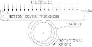
Empirical methods like the classic CEMA formulation give good results when the design parameters are close to the experimental data from which the empirical formulations were derived. The classic CEMA method works fairly well even outside the experimental parameter range as long as the temperature is above zero and the belt rubber compounds are similar to the compound tested by Penn State in 1954. Because of the inherent limitations of empirical methods, a number of researchers have proposed semi-analytical and theoretical methods of predicting conveyor power consumption [7 - 10].In 1989 Conveyor Dynamics, Inc (CDI) commissioned two overland conveyors at the Channar Mine in Western Australia. Before commissioning this system, a number of major firms predicted that CDI had undersized the motors. After commissioning, CDI showed that the friction factor on the straight overland was only 0.0098 and the friction factor on the horizontally curved belt was 0.011 [11]. Later, the friction even fell to 0.0085. This marvelous result (less than half of the recommend DIN standard base friction) surprised everyone. The conveyor hadexceeded even CDI’s expectations, and convinced CDI to invest in developing a new method of predicting conveyor power.In 1990 Syncrude Canada realized that they had a number of issues with their conveyors stemming from the fact that their power consumption was vastly different from the CEMA predictions. To solve this problem, Syncrude awarded CDI a contract to invent a new theoretical model of conveyor power consumption capable of explaining the strange behavior they observed in their conveyors [12]. Our earlier model is described by Nordell in [13].The model we use now is a two-dimensional plane-strain semi-analytical model that allows us to engineer the most energy efficient conveyors operating in the world today including the worlds’ longest single flight conventional belt conveyor [14].In 2006 Overland Conveyor Co (OCC) proposed a simpler idler-belt interaction model but instead of a 2D plain stress model, they chose a 1D spring-dashpot model which, unlike the CDI formulation, neglects shear stress [15].Both CDI and OCC’s indentation models are classified as “Small Sample Indentation Tests” (SSIT) because they require the engineer to measure the viscoelastic properties of a “small sample” of rubber used in the bottom cover of a conveyor belt. The rubber is characterized using master curves of G’ (elastic stored energy) and G” (energy lost to heat) as functions of time, temperature, and frequency. Both methods predict the indentation losses in a uniformly loaded slice of belt (shown in Fig. 1 with width ∂z). In this figure the belt is not rebounding as fast as it compresses. This causes the rubber entering the idler roll to push harder on the roll than the rubber leaving the idler which in turn, creates a force (indentation loss) that resists belt motion.
The total resistance to motion is the sum total of the resistances contributed by all the ∂z thick slices in a belt cross section. The pressure on each slice depends on the load the slice is supporting, the stiffness of the belt, and the trough angle.CDI’s methodology remains largely a trade secret. OCC’s methodology was incorporated into the sixth and seventh editions of The Belt Book. However, programming small sample methods is a daunting task for many users of the Belt Book, and while several companies, including CDI, sell expensive software packages to perform these calculations, many designers still prefer to work with spreadsheets and programs they created themselves. For this reason, the CEMA-6 and CEMA-7 small sample methods are quite controversial.
The Large Sample Method
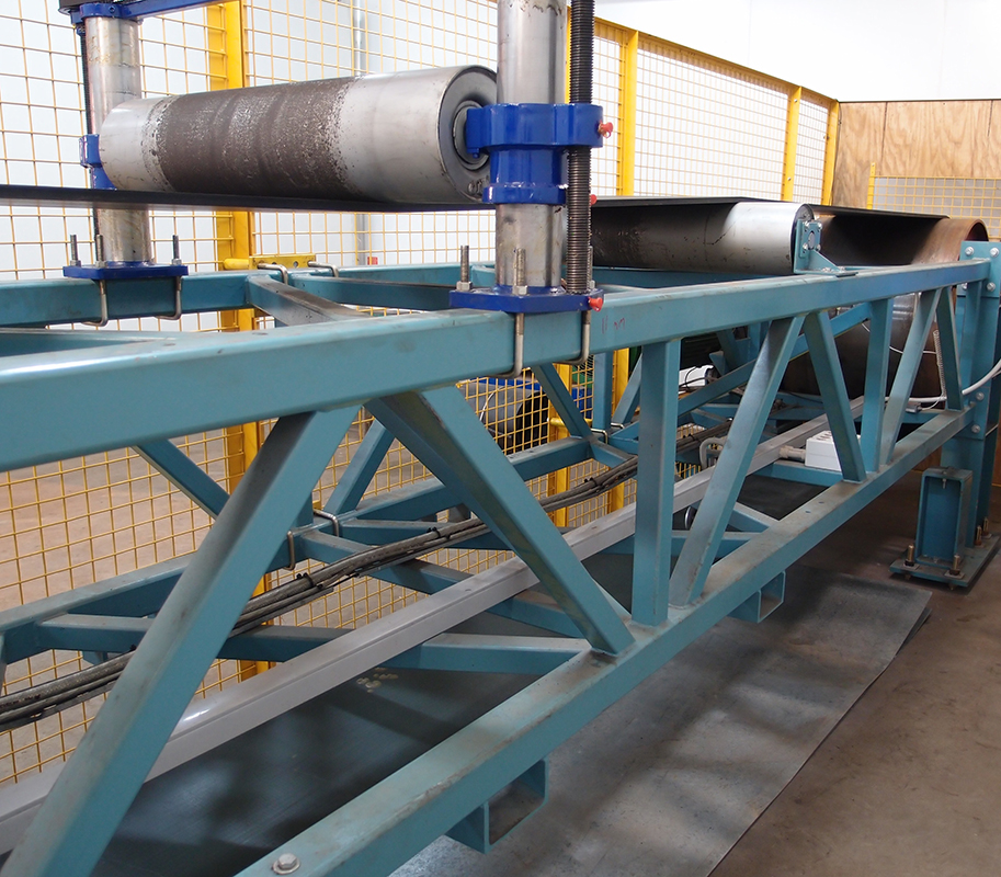
Before developing our Small Sample Method, CDI and Syncrude Canada built a number of large scale test machines to study the behavior of their conveyors. Two of the machines we built are shown in Fig. 2. Our indentation loss machine directly measured indentation losses for different temperatures, pressures, and speeds. Since the pressure on the idler is uniform, one can divide the measured resistance by the idler roll length to get values with units of [Force/Width]. This is exactly the value calculated using the small sample method.

indentation loss test machine (right).
We could avoid all the small sample method calculations using machines like this, but these machines require a “Large Sample” of rubber which is expensive to obtain, handle, and store. Having proven that our small sample method yielded the same results as our large sample indentation test (LSIT) machine, we decommissioned the device.Recently, interest is again growing in LSIT machines. Hannover University in Germany is operating one such machine [17]. To develop new types of low rolling resistance (LRR) belting, CDI, Laing O’Rourke, and Veyance Belting jointly contributed to a grant which the University of Newcastle used to build the large sample test machine shown in Fig. 3 [18]. Both of the Hannover and the Newcastle machines are essentially short flat belt conveyors with uniformly loaded idler rolls creating indentation losses.
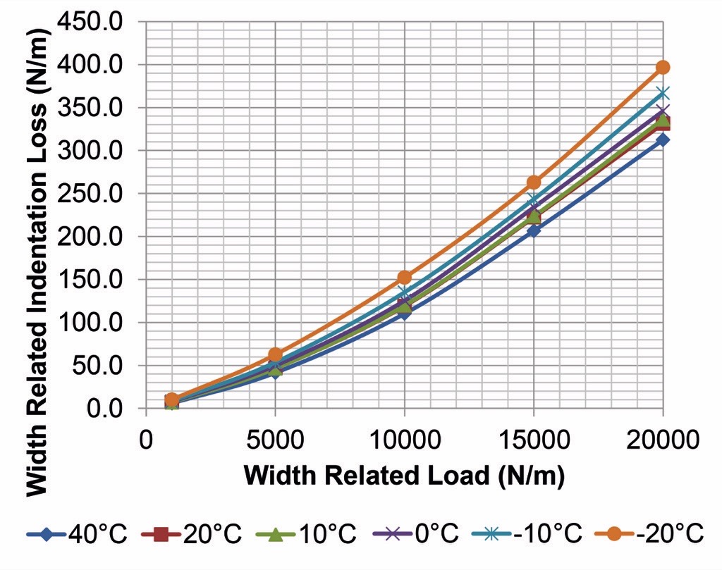
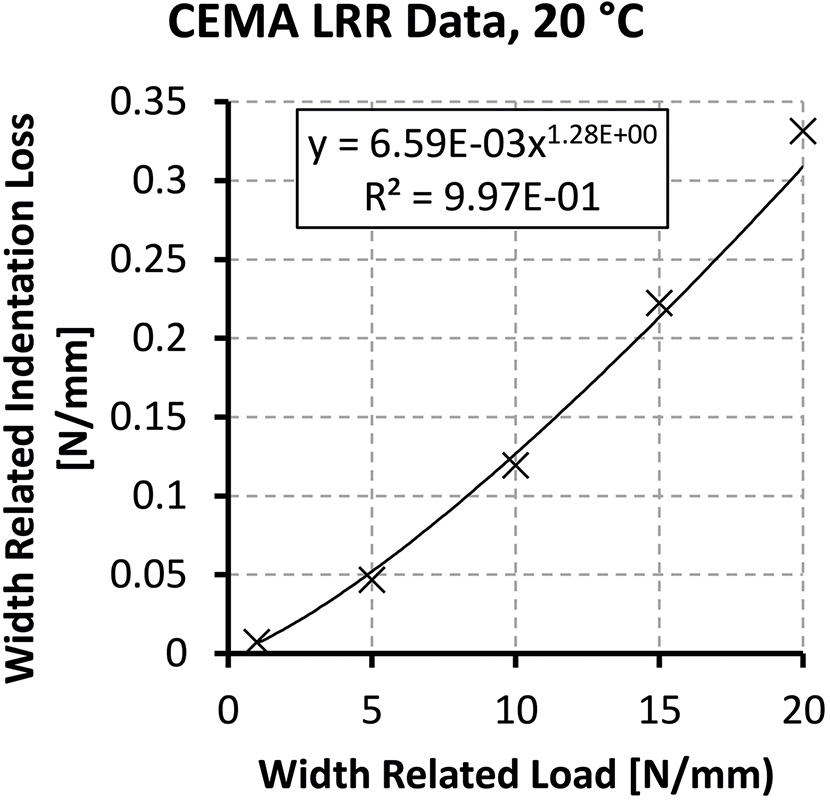
The drag measured by large sample test machines is much easier for laymen to understand than master curves produced by small sample test machines. For this reason, mine owners are beginning to require belt manufacturers to submit samples of their LRR belts to large sample testing laboratories so that owners can compare the efficiencies of these belts. Results from LSIT tests are making their way into the industry at large. In recognition of this fact, the German Industrial Norming committee (DIN) recently defined a new standard, DIN-22123:2012, to standardize LSIT test procedures and reports.DIN 22123 specifies that LSIT reports shall include a list of “Width Related Load [N/mm]” (WRL) which is the applied load divided by test belt width, and a resulting “Width Related Indentation Rolling Resistance [N/mm]” (WRIRR) which is the indentation resistance divided by test belt width. Sample data from a typical LSIT appear in Fig. 4. The appendix of DIN 22123 recommends fitting each temperature line on this plot with the function “WRIRR = a · (WRL)b”.
Another function could be used, but DIN’s function is simple and passes through (0,0) which is critical. To compute the power loss over the cross-section of a real conveyor with the same idler diameter, temperature, and belt construction of the test, the engineer:Step 1: Determines the distribution of load on the idlers at the interface between the belt and the idlers — WRL(z) = q(z).Step 2: Fits the WRL and WRIRR data from the LSIT report with a function that relates load to resistance, such as
Step 3: Computes:
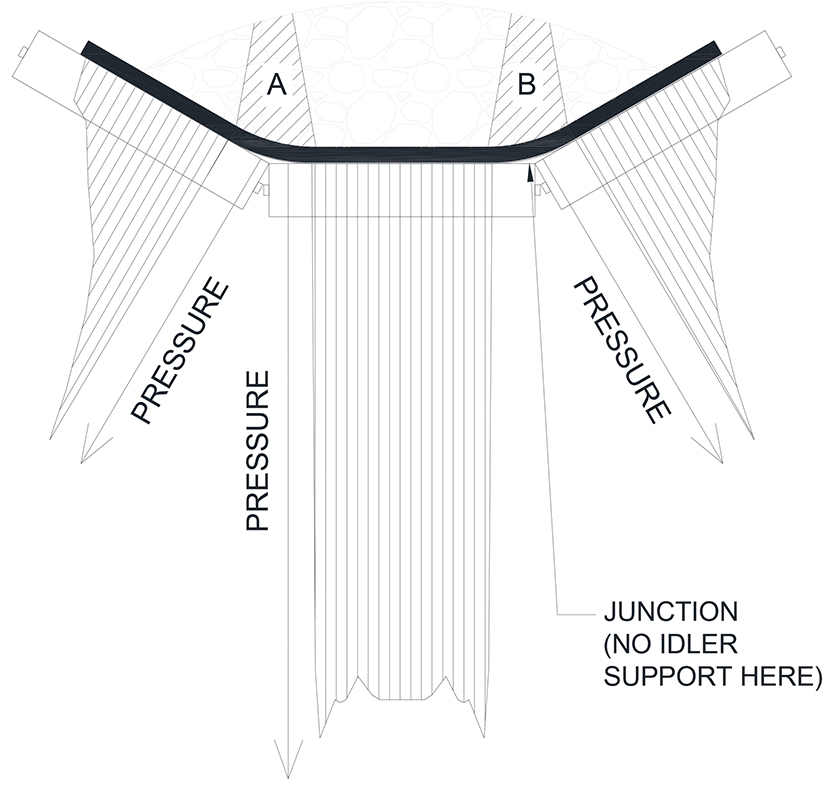
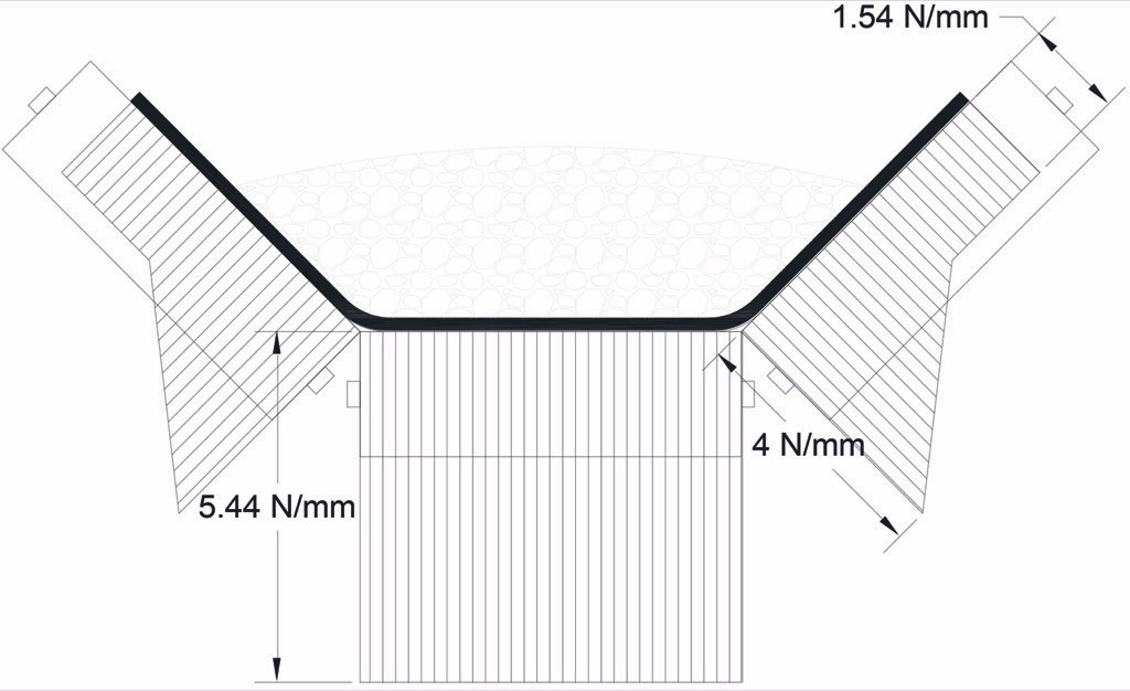
The pressure distribution on an idler roll, q(z), is not trivial. Fig. 5 shows the pressure distribution Grabner [16] measured on typical carry side troughed belt idler rolls in a straight section of belt. Since the belt below the junction regions ‘A’ and ‘B’ does not touch the rolls, the load in these regions is supported by the belt at the edges of the junction. While the integral of the force in the vertical direction must equal the weight of the belt plus material, the pressure distribution is different from a hydrostatic distribution because bulk materials, unlike fluids, support shear. This means that centrally located particles can transfer some of their weight to the wing rolls through friction forces. The effect is particularly pronounced when the belt is moving, because the sides of the trough compress into the material when the belt enters the idler trough and relax when the belt leaves the idler trough.
Large Sample Integration Example
For this example, we will predict the indentation losses of a carry side idler set in a straight, horizontal, section of a conveyor with the following parameters:
| Bw | = | belt width = 1600 mm = 1.6 m | |
| γ | == | bulk density = 800 kg/m³7840 N/m³ | |
| v | = | belt speed, = 7.5 m/s | |
| Q | = | tonnage= 4860 t/h = 13,230 N/s | |
| φs | = | surcharge angle, = 15 degs | |
| β | = | trough angle = 45° (carry), 30° (return) | |
| Si | = | carry idler spacing = 2 m (carry), 8 m (return) | |
| D0 | = | idler diameter = 194 mm (carry), 178 mm (return) | |
| Wb | == | belt weight = 39.5 kg/m387.1 N/m | |
| RLC | = | center roll length = 593.6 mm | |
| T | = | temperature = 20°C | |
| h0 | = | bottom cover thickness = 6 mm | |
| Bottom cover rubber type: LRR Rubber | |||
Mathematical formula for the pressure distribution on an idler roll can be quite complicated [19] and are beyond the scope of this paper.To simplify our example, we shall adopt the distribution used by Tapp [20]. For a 45° trough, Tapp evenly distributes 75 % of the load in the center roll, and allocates the remaining 25 % of the load to the wing rollers using a triangular distribution.Accordingly, we compute q(z) for the carry:
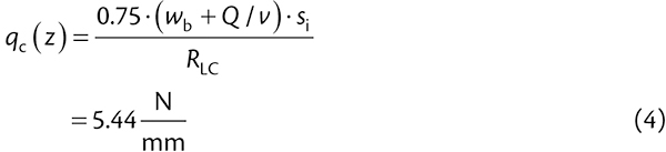 |
The pressure of the belt against the wing roll is:
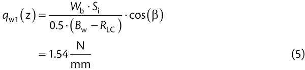 |
Note: Tapp’s distribution assumes a hydrostatic pressure and thus, includes no cos() term. In reality, Tapp overestimates the material pressure on the wing roll which is clear if we sum the loads measured by Grabner.To calculate the pressure distribution on the wing roll we first compute the distance from the junction to the edge of the material. The Belt Book includes a complicated, accurate formula to compute the distance from the edge of the belt to the edge of material. Using this formula we compute this edge distance, Bwe = 193 mm. From edge distance we compute the distance from the junction to the edge of material: Lwm = 0.5 · (Bw - RLC) - Bwe = 310. From this we compute the wing roll pressure distribution:
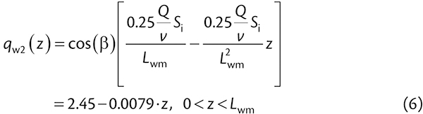 |
Combining qc(z), qw1(z), and qw2(z) we get the pressure distribution shown in Fig. 6.
The pressure levels in this figure are fairly typical of the pressures found in conveyor belts. A good range for large sample test data is between 0.5 N/mm and 9 N/mm. Some laboratories [17] are currently testing large samples at pressure several times higher than this. The LSIT data in CEMA-7 combines results from several sources and thus includes a much wider range than the engineer is likely to find on trough belts operating in the field. Fig. 7 shows a plot of the 20°C LRR data from CEMA-7 fitted with the formula Eq. 2. According to CEMA-7, for an LRR belt at 20°C, ‘a’ = 6.59 · 10-3 and ‘b’ = 1.28.
Since the CEMA test data was measured on a belt with a 7 mm bottom cover and an idler roll diameter of 219 mm, we must scale the CEMA results to model our conveyor. To estimate how much this friction would change if we retested the sample using a different idler diameter and/or belt thickness we multiply constant ‘a’ by the following equation [13]:
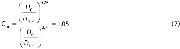 |
where:
| Htest | = | belt bottom cover thickness used to produce the LSIT test | |
| DTest | = | diameter of the idler roll used to produce the LSIT data |
Finally, we substitute Eqs. (4), (5), and (6) into Eq. (2) and integrate the result over the width of the belt as follows:
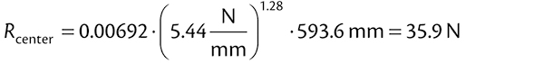 |
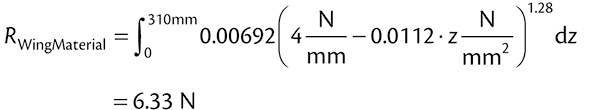 |
Thus, using this methodology, the total indentation loss on an idler set is:
Transforming Large Sample Test Data for Use in theClassic CEMA Formulation
For more than half a century conveyor designers used simple friction factor based formulas like Eq. (1) to design conveyors. Experienced conveyor engineers have a “feel” for what friction factors are reasonable on various types of systems, and often the first question auditors ask conveyor engineers is, “what friction factor did you use?”To get a friction factor, we could simply divide Eq. (3) by the total load on the idler. However, by reconditioning LSIT results in terms of friction factors we can use them in formulas that conveyor engineers are familiar with. This was one of the primary goals of the committee charged with writing the LSIT section in CEMA-7.To transform the C and WRIRR into a new friction factor we simply divide the resistance by the applied load and multiply by Chr:
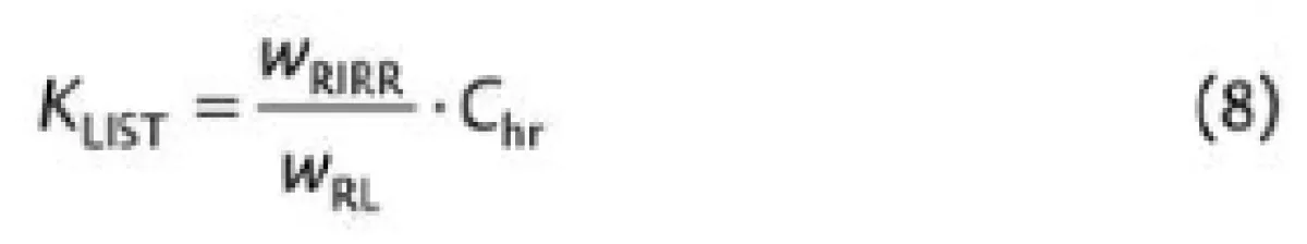
|
The question then becomes, “which WRL should I use to select a WRIRR?” The LSIT Section in CEMA-7 recommends selecting the WRIRR which corresponds to the average load on the belt cross section:
However, since the relation between WRL and WRIRR is nonlinear, we need to correct this friction to account for the nonlinear pressure distribution. The small sample method in CEMA-6 and CEMA-7 has the same problem. OCC did not provide CEMA with a pressure distribution and did not describe how to perform the integration discussed in the previous section. Instead, users of the small sample method in CEMA-7 apply the following correction factor to the small sample method results:
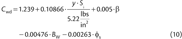 |
Where bulk density has units of lbf/in³, angles are in degrees, belt width has units of inches, and idler spacing has units of inches. The author of this paper has no idea how this formula was derived, but to maintain consistency the writers of CEMA-7 LSIT also recommend using the same formula to scale LSIT results. Accordingly, we can define a new friction factor:
The indentation loss is then calculated using the following formula:
For the example conveyor in the previous section, WRL_AVG = 2.69 N/mm, KLSIT = 0.00913, Cwd = 1.113, Ky1 = 0.0103To calculate the drag on a single idler set we set I = Si. Thus, using this friction factor based method, we predict that the drag is:
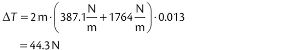 |
Comparison with Field Measurements
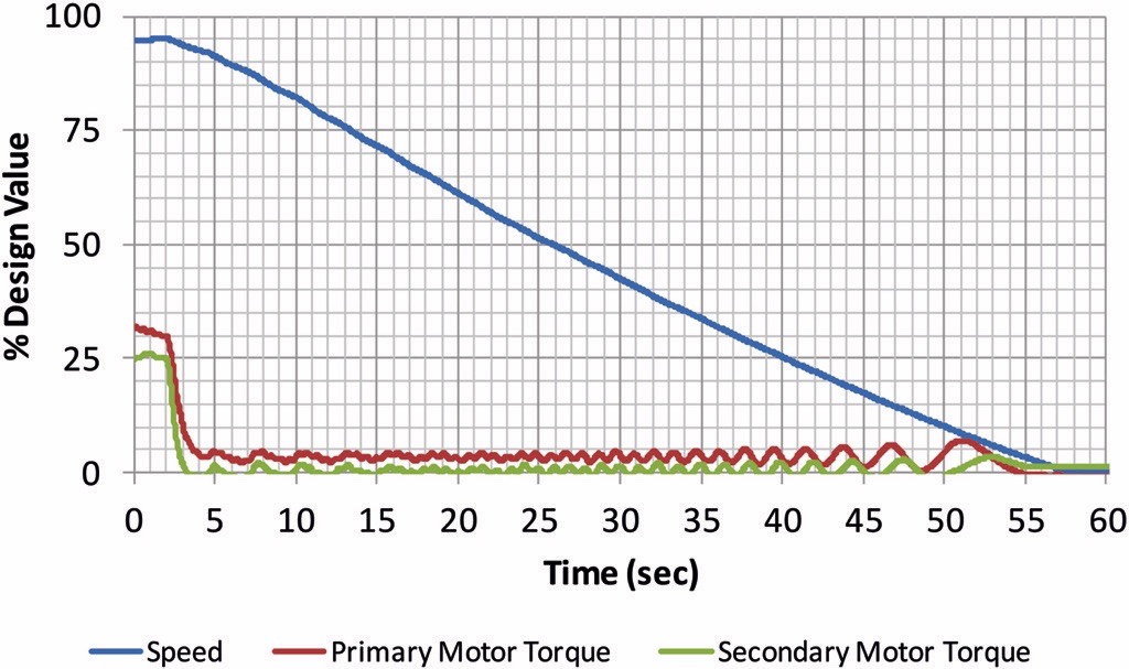
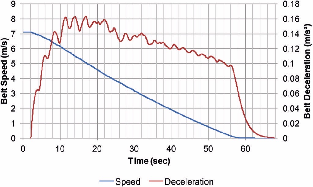
While commissioning the Dahej Overland Conveyor in India [21], the author used strain gauges to measure the drive torque during the exact scenario described in the previous two sections. The author also measured the torque on the motor shafts while the belt ran empty. Fig. 8 shows the torque on the shaft and speed of the belt during an empty drift stop. 26 % motor torque is equivalent to a drag of 35468 N. As the conveyor slows, there is less friction retarding conveyor motion and this is reflected in the deceleration curve shown in Fig. 9. Using these curves and Newton’s 2ndlaw we compute that mass of the empty conveyor is 196546 kg.
Although the weigh scale was not operational while CDI was present at site, we repeated the drift stop when the belt had enough load to require 63.2 % of motor torque. This test showed that 4860 t/h require 63.2 % motor torque which is equivalent to 85885 N of drag. There are 817 idler sets on the carry side of the Dahej conveyor and thus the additional drag created by loading material on the belt is (85885 N – 35468 N) / 817 sets = 61.7 N/set.The 61.7 N/set figure includes trampling losses, load dependent idler losses, and flexure losses. Using our proprietary flexure and trampling losses method, CDI predicts the 11 % of the losses at Dahej resulted from trampling and flexure. If so the indentation losses were less than 55 N/set.Further, the LRR belt data presented in CEMA is an LRR rubber compound made by an American manufacturer. The LRR rubber at Dahej is a different compound manufactured by a German company so the CEMA LSIT data does not really apply. The comparison is not perfect but these values are all in the right ballpark for an LRR belt.
Conclusions
Computing conveyor power using theoretical models involves a substantial amount of advanced mathematics, physics, and material science. Empirical methods like the classic CEMA method offer time tested simple methods of estimating a conveyor’s horsepower requirement as long as conventional rubbers are used in the belt. Large sample indentation tests allow designers to derive new empirical power consumption formulas and predict the behavior of modern rubbers with classical methods of conveyor design.The indentation loss prediction using the method described in CEMA-7 is simple to implement in a spreadsheet and very similar to the classic CEMA horsepower equation. However, the derivation of CEMA-7’s formula for Cwd is not known to the author. Field measurements sug-gest that CEMA-7 works well in somescenarios, but without the derivation of Cwd, it is difficult for the author to determine the range of conditions for which CEMA-7 applies. The latest editions of CEMA are a step forward for the industry, and will allows designers to estimate the savings LRR rubbers can yield for operators.Still, the methods presented in CEMA include a number of simplifications and approximations which impact their accuracy. CDI recommends that designer apply at least a 15 % margin on top of any CEMA-7 based design. Internally, we do not plan to adopt the CEMA approach ourselves. We will continue to use the more detailed theoretical models we developed for Syncrude.
References:
- Conveyor Equipment Manufactures Association, Belt Conveyors for Bulk Materials, 7th Edition, Naples, Florida USA: Conveyor Equipment Manufactures Association, 2014.
- Conveyor Equipment Manufacturers Association, Belt Conveyors for Bulk Material, 1st Edition, Boston: Cahners, 1966.
- German Industrial Standard DIN-22101: Belt Conveyors for Bulk Materials, 1982.
- Asman, A.W.: Belt Conveyor Power Studies, AIME Transactions, vol. 217, pp. 216-220, 1961.
- Breuil, F., Radomsky, G. and Cooper, P.: Method and Apparatus to Measure the ‘Conveying Resistance’ of Belt Conveyors, in AIME Annual Meeting, New York, 1956.
- Asman, A.W.: More From Belt Conveyors, Coal Age, vol. 60, no. 12, pp. 66-68, 1955.
- Hunter, S.H.: The Rolling Contact of a Rigid Cylinder with a Viscoelastic Half Space, Journal of Applied Mechanics, vol. 28, no. 4, pp. 611-617, 1961.
- Spaans, C.: The Indentation resistance of Belt Conveyors, Delft university of Technology, The Netherlands, 1978.
- Spaans, C.: The Flexure resistance of Belt Conveyors, Delft University of Technology, The Netherlands, 1979.
- Jonkers, C.: The Indentation Rolling Resistance of Belt Conveyors, Fördern und Heben, vol. 30, no. 4, pp. 312-317, 1980.
- Nordell, L.K.: The Channar 20 km Overland- A Flagship for Modern Belt Conveyor Technology, Bulk Solids Handling, vol. 11, no. 4, pp. 781-792, 1991.
- Melley, R.; Bland, S. and McTurk, J.: Optimization of Oil Sands Conveying Through Field Measurements, Mining Engineering, vol. 45, no. 3, p. 11, 1993.
- Nordell, L.K.: The Power of Rubber- Part I, Bulk Solids Handling, vol. 16, no. 3, pp. 333-341, 1996.
- Stevens, R.: Belting the Worlds’ Longest Single Flight Conventional Overland Belt Conveyor, Bulk Solids Handling, vol. 28, no. 3, pp. 172-181, 2008.
- Rudolphi, R. and Reicks, A.: Viscoelastic indentation and resistance to motion of conveyor belts using a generalize Maxwell model of backing material, Rubber Chemistry and Technology, vol. 79, no. 2, pp. 307-319, 2006.
- Grabner, K., Grimmer, K.-J. and Kessler, F.: Research into Normal-Forces between Belt and Idlers at critical Locations on the Belt Conveyor Track, Bulk Solids Handling, vol. 13, no. 4, pp. 727-734, 1993.
- Kropf-Eilers, A., Overmeyer, L. and Wennekamp, T.: Energy-Optimized Belt Conveyors - Development, Testing Methods and Field Measurements, Aufbereitungs Technik, vol. 49, no. 9, pp. 25-34, 2008.
- Wheeler, C. and Munzenberger, P.: Indentation Rolling Resistance Measurement, in Beltcon 16, Johannesburg, South Africa, 2011.
- Spaans, C.: The Calculation of the Main Resistance of Belt Conveyors, Bulk Solids Handling, vol. 11, no. 4, pp. 809-826, 1991.
- Tapp, T.: Energy Saving Trough Idler Technology, Bulk Solids Handling, vol. 20, no. 4, pp. 437-449, 2000.
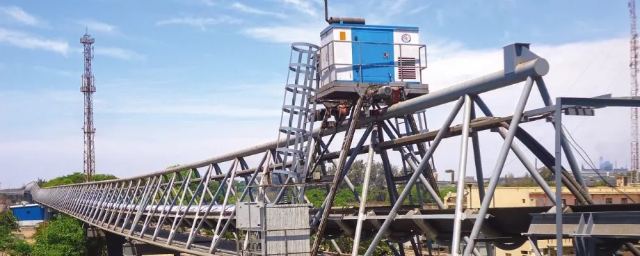
- Jennings, A., Bhansari, J., and Shah, K.: India’s First Elevated, Triangulated Gallery Overland Conveyor, Bulk Solids Handling, vol. 33, no. 6, pp. 24-27, 2013.
| About the Author | |
| Andrew JenningsPresidentConveyor Dynamics, Inc., USA |
■

