Dear Teus,

the location of the operating point of this pneymatic conveying installation (50 t/h fly ash) is shown in the dilute area of my state diagram, and it forms together with the operating conditions of all the other industrial installations the diagram's sceleton.

Kind regards

ManfredH ■

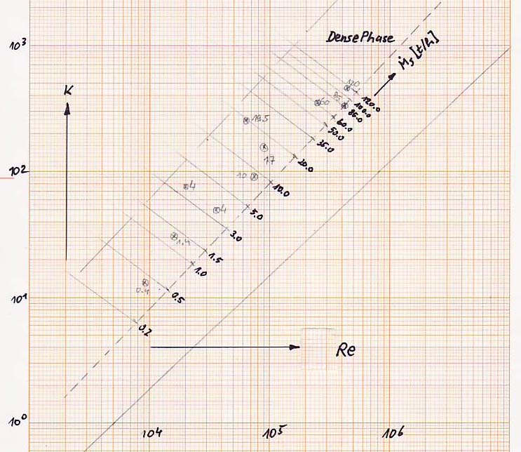
The state diagram shows at the abscissa the well known dimensionless Reynolds number and at the ordinate a dimensionless expression from my theoretical work on the turbulent gas flow in pipes; in this discussion I will name it K number. K contains mainly the pressure loss and the length as well as the diameter of the pipe and the dynamic viscosity of the gas. The diagram is an implied presentation of the physical parameters and makes an iterative way of calculation necessary.

The main reason for such a diagram was, to show this mess of published and discussed conveying conditions in industrial installations in a clear and universal way. I found an abundant number of published data sets as well as scientific investigation results, which I could incorporate into the coordinate system in order to form the sceleton of the state diagram. With the help of the data I could define the dilute phase area as well as the dense phase area. In the dilute phase area there are two characteristic conveying states, represented by the line of minimum pressure loss and by the so called shoking line at the boundary of the instable transition area. Another characteristic conveying state is represented by the boundary line of the dense phase area, that I believe to have determined now with the help of the data of installation No. 23 in the list. Furthermore I extracted the in dense phase mostly used pipe diameter for the industrial installations as ratio to the bulk solid mass flow.

To ease the calculation the current software program suggests a usable value for the pipe diameter. Furthermore there are suggestions for the coordinates of the three characterisic conveying states on the basis of the design data. These values are calculated by simple equations for the three straight lines in the diagram. For all the other possible operating points one has to read the coordinates from the diagram. The upper line of maximum mass flow is only hinted, but it can be easily precised, as I described above.

The dilute phase calculation uses the suggested pipe diameter for a direct calculation, which is corrected in case of deviations from this value. In case of larger particle diameters the gas velocity is sometimes higher than calculated for the minimum pressure loss: 18 m/s instead of 15 m/s for installation No. 18 (2 mm) of the list; 27 m/s instead of 11 m/s for No 17 (25 mm); 35 m/s instead of 21 m/s for No 24 (2.5 mm). For the installation No 21 (4 mm) operating data and calculated values are identic. Interresting is, that the installations No 3 and No 10, because of the particle size predestinated for dense phase conveying, are situated at the boundary line of the dilute phase.

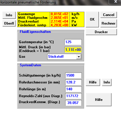
The incorporated dense phase operating points spread over the whole area, offering the possibillity to estimate the lines of equal bulk solid mass flows. The maximum mass flow was 19.5 t/h. Fortunately the installation No 23, described in bulk-online, now gave the opportunity to determine the boundary line more precisely, because this operating point lies almost exactly on the boundary. For the gas temperature of 125 °C and the mass flow of 85 t/h together with the program's coordinates for the boundary line (because of the improvement no longer identic with the diagram's) the calculated values are: 7060 kg/h for the gas flow and 1.66 bar for the pressure drop. For the troughput of 100 t/h discussed in the thread the calculated values are: 7860 kg/h and 1.92 bar, so that the actual compressor performance seems to provide no scope for such an increase; the power limit seems at least to have been reached.

In contrast to the fine materials, for which one dense phase conveying systems usually use, lies the particle size of the installation No 22 in mm range. Nonetheless, the bulk solid is conveyed according to the disclosures without any problems at the given dense phase conditions (Re / K = 250,000 / 350), except in 90° bends, when the pipe, in case it rises vertically upwards, begins to vibrate.

The questions remaining: what are the right operating points in dense phase conveying? Why are the operating points in dense phase so different? How should look a scale-up for comparable conveying conditions?

*) Regarding the horizontal pneumatic conveying installations with vertically orientated pipe sections I normally take them into consideration by increasing their lengths by a factor between 1.5 and 2.

**) "The state diagram is independent of the conveyed material and therefore independent of material conveying properties, s.a. suspension velocity and the collision loss factor." This remark by Teus is correct, and I have nothing to say on this subject. You have to evaluate my presentation yourself. ■

Dear Tois!

In case of Krambrock's, diagram for maximum mass flows of PE granules I have the impression that in this case the bulk solid can be conveyed at any operating point. But it is correct, that the question for the right operating point cannot directly be answered by the state diagram. The only way is, estimating a pipe diameter in dependence of the solids mass flow as well as the suspension- or floating-velocity of the particles (I refer to your explanations in the thread "Conveying Air Velocity": https://forum.bulk-online.com/showth...g-Air-Velocity) and choose an appropriate operating point on the associated line of equal mass flow. In case of large particle sizes there could possibly help an additional guidance: pipe diameter at least 30 X particle diameter because below this value for instance hopper discharges are being unfavorably influenced.

But let us make it not too complicated. The main aim of the diagram was, to show the positions of operating points from installed conveying lines in order to be able to predict changes of the operating conditions. And may I remind you of the installation No 23. Taking into account the high gas temperatur (that leads in my calculation to a high increase of pressure loss), there was from my point of view no scope for an increase like your calculation resulted.

By the way, there aren't any code-related problems running the software routine. Input and output look like this:

Kind regards

ManfredH ■

The fact that in many industrial installations for the conveying of fine-grained bulk materials the operating conditions do not lie in the dense phase area but on the boundary of the dilute phase area has surely certain reasons: the conveying velocity, on the one hand, is as low as possible, on the other hand is the influence of the bulk material properties on the conveying behaviour, difficult to estimate for the dense phase state, not so decisive.

ManfredH ■

This is a sketch of the dense phase part of my state diagram after the relevant conveying installations from the bulk-online threads have been taken into account. The endpoints of the lines of equal bulk solids throughputs are calculated by my software program.

href="https://forum.bulk-online.com/attachment.php?attachmentid=32812&d=1337071246" id="attachment32812" rel="Lightbox74475" target="blank">■

To understand the origin of the dimensionless Number "K" (Ratio between tube diameter and wall-related "mixture length" or "Mischungsweglänge" by Prandtl) used for the state diagram, see my interpretation of the turbulent pipe flow and the resulting equations for the calculation of pressure loss and heat transfer. Sorry, the text is in German, but the decisive equations (6-23) and (6-24) as well as (6-37) are easy to find. You can retrieve the document under the following link:

https://skydrive.live.com/redir.aspx...M0fIsQJ09T20A ■

Originally Posted by Teus Tuinenburg

Dear Manfred,

I am still puzzling the meaning of your State Diagram.

In the file KFaktor.pdf there is the formula (6.23):

∆p=0.097*Re^(1.8)*(^2*L)/(*D^3 )

or

1=(∆p**D^3)/(0.097*Re^(1.8)*^2*L)=√(1/(0.097*Re^(1.8) ))*√((∆p**D^3)/(L*^2 ))

In the State Diagram, the formula for the ordinate is:

y=0.0015*√((∆p**D^3)/(L*^2 ))

Combined:

y=0.0015*√((0.097*Re^(1.8))/1)

resulting in:

y=4.67*Re^(0.9)

The plot of y = function(Re) is a straight line in a logarithmic coordinates system.

The plots, outside of this straight line, must be representing a pneumatic conveying installation, where the pressure drop is influenced by the presence of material.

(In the state diagram, as presented in this thread, there are Zenz like curves noticeable)

Can you explain the background and the meaning and usefulness of your approach?

BR

Teus

Dear Teus,

from the formal point of view I can only say the following: the expression D/lw (K-Faktor) as ordinate is the expression for Re^0.9 from eq. (6-24) substituted in eq. (6-23).

Regarding the usefullness of my state diagram I think to have made this clear by discussing the diagram as well as different industrial conveying installations. With the help of the physically based dimensionless K-faktor I hope to provide a clear and universal overview over the operating conditions of industrial installations and to answer some on bulk-online often asked questions, for example the extent of the different conveying regimes, the characteristic conveying states, or the influence of the temperature on the pressure loss. My software allows quick estimations.

Verifying the different industrial installations under the conditions of my state diagram, I could not discover any clear influences of bulk-solids properties.

Regards

ManfredH ■

Regarding the influence of the gas temperature you neglected the effect on the dynamic viscosity in the K-Faktor. And what is wrong on a dimensionless Number that is based on a verified physical model for the turbulent pipe flow. Otherwise I cannot understand, that your are ignoring all the calculation results presented by me. I wonder, if you had ever been so critical with the Zenz-diagram, that you constantly uses. I am not pleased about this discussion, that in my opinion is applied to undermine my original intentions. So, I will retreat myself.

Regards ■

In order to return to the practical side of my state diagram I will present now some data from industrial installations working at high temperatures. The installations are described under the following internet adress: http://www.enviro-engineering.de/pdf...nwendungen.pdf

( ) = calculated values, µ = loading ratio

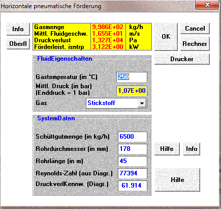
1. Like in other installations with similar particle sizes the conveying condition is dilute phase working at a gas velocity factor of 1.6 higher than the calculated velocity of minimum pressure drop. The extrapolation from the calculated point of minimum pressure drop gives the values of 100,000 and 25 for Re and K. The calculation looks like this.

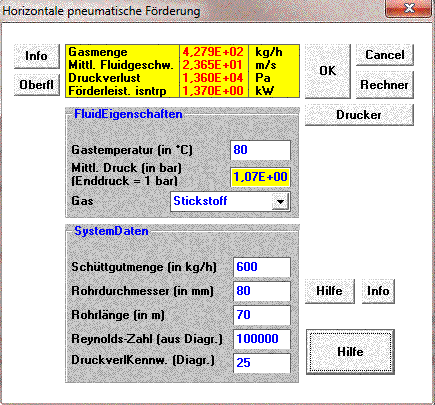
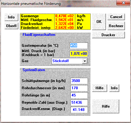
2. The Data of this installation are for a gas temperature of 250 °C. The bulk solid flow at that temperature is 6.5 t/h and is considered surprisingly high. The calculated pressure drop for the dense phase boundary is 0.133 bar at a gas flow around 1000 kg/h. Look the following calculation sheet.

The following sheet shows the situation at the design temperature of 450 °C and an equal pressure loss. The gas flow is in this case under 900 kg/h. The bulk solid flow is significantly lower and correspond to the design value of 3500 kg/h.

3. Once more the data set from the following bulk-online thread:https://forum.bulk-online.com/showth...peline-Pigging. The installation gave the opportunity to determine the boundary line more precisely, because this operating point lies almost exactly on the boundary. For the gas temperature of 125 °C and the mass flow of 85 t/h together with the program's coordinates for the boundary line (because of the improvement no longer identic with the diagram's) the calculated values are: 7060 kg/h for the gas flow and 1.66 bar for the pressure drop. For the troughput of 100 t/h discussed in the thread the calculated values are: 7860 kg/h and 1.92 bar, so that the actual compressor performance seems to provide no scope for such an increase; the power limit seems at least to have been reached.

From given cause let me add, that this thread was intended to show published data of industrial installations, to discuss them under the conditions of my state diagram, and to improve the relationships if possible. This thread was not intended to compete to any other (possibly not comparable) calculation model. So, I was not waiting for great declarations in favour of ........., and I was not waiting for instruction on physical matters. ■

Of course, I asked myself, too, why the bulk properties in my state diagram are not visible, and why friction-factor-bounded interpretations obviously are failing. An explanation for that could be, that the state diagram is a cumulative presentation. Influencing factors like friction, acceleration and gravity (and their contributions) as well as the resulting flow pattern such as plug flow and dune flow hide themselves in the total pressure loss (or K-factor). I tried and failed to discover (and to extract) relations between the map and parameters like particle size, SLR or particle density. I found data of different installations that fit into the state diagram without any problems and independently of the specific bulk solid data.

A sort of analogy can one find in simplier functioning fluidized beds. The pressure loss depends only on the mass of bulk solid, not on its characteristics, and remains constant with increasing gas flow. The respective flow condition and bulk solid behaviour in the fluidized bed are only indirectly visible for example in the gas velocity, in the hight of the expanded bed, as well as in the heat transfer and in the results of catalytical gas phase reactions. ■

Originally Posted by Teus Tuinenburg

Dear Manfred,

A point in the state diagram is given by:

SQRT[(dp*D^3*rhogas^2)/(etagas^2 * L)] = SQRT(SLR * K/2) * Re

(see derivation in reply #17 of this thread.

In the state diagram, the y-axis is noted as:

SQRT[(dp*D^3*rhogas^2)/(etagas^2 * L)] = 0.0015 * Re

hence,

SQRT(SLR * K/2) = 0.0015

SLR is an operating variable

K is a material variable

By setting the value to 0.0015, all materials are treated as the same material.

By calculating the value “SQRT(SLR * K/2) = 0.0015”, the operating point shifts in the state diagram to a material- and operating condition related point.

I believe that the structure of the state diagram is now explained.

As to the analogy to fluidized beds, a must admit that I have no relevant experience with.

Have a nice day

Teus

Hi, Mr. Tuinenburg!

Sorry, but what you are expressing leads in my opinion away from the real essence of the state diagram . Not the possibly neglected influence of bulk solid characteristics is the main thing. First and foremost lies the importance of the state-diagram in its presentation of similarity laws, so that different conditions in pneumatic conveying are comparable. In this context it would also be possible to reformulate the K-factor on the basis of indicators like Euler number, Froude number and Galilei number.

In fact, for the dilute phase it was necessary to consider an influence of the tube diameter. However, as I stated earlier, I have observed nothing of the sort for the dense flow.

And what is the meaning of "the same materials", and what are their characteristics, and how can the (up until now invisible) influences be determined and taken into account.

Regards

Manfred ■

I'm really not a great physicist, and it is the first time for me that I am in such a situation. But the mathematical efforts of Mr. Tuinenburg regarding my state diagram gave me reason to point out misunderstandigs on which his efforts are based.

The only physical elements of the diagram are the abcissa and the ordinate. Together with the straight line on the right side they represent the equation for the turbulent pipe flow as a result of a verified physical model.

All the other lines in the diagram are representing measurement results. One can try to interpret their physical meaning, one can try to find locations for spezific conveying states and describe them graphically or mathematically, and, if possible, one can use verified results as similarity laws.

Regarding the whole mathematical efforts by Mr. Tuinenburg the conclusion is: without any specific measurement results or specific interpretations of measurement results it is not possible to develop the state diagram any further or to discuss for example influences of the bulk solid characteristics.

And that's it. ■

Der theoretische Hintergrund zur pneumatischen Förderung ist Teil meines bei epubli erschienenen ebook

Fluidisieren von Schüttgütern,

das für begrenzte Zeit innerhalb von Deutschland unter folgendem Link versandkostenfrei bestellt werden kann.

http://www.epubli.de/shop/autor/Manfred-Heyde/3168

Dafür gibt es folgenden Gutscheincode:

epubli-SOMMER2012

Der Gutschein hat einen Wert von 4,95 € und ist bis 15. Oktober 2012 gültig. ■